Can a Neural Net Learn the Quadratic Formula?
Yes, but there’s a catch!
The Problem
At first glance, this problem seems trivial. Neural nets are sophisticated technical constructs capable of advanced feats of machine learning, and you learned the quadratic formula in middle school. But an interesting property of classifiers was revealed trying to solve this issue. So please, bear with us for a little, and we’ll show you why this matters.
Let’s start by more precisely defining the problem:
Given a polynomial p(x) = a⋅x² + b⋅x + c with real coefficients and roots (such that a ≠ 0 and b² ≥ 4c), can we train a neural net to output the roots of p?
Learning Roots
We first made sure that a neural net could be trained to approximate the square root function. This was a natural place to start, since solving of the square root function is needed to learn the quadratic function. If a neural net couldn’t learn it, we had no hope of solving the quadratic formula. We used PyTorch to define a simple neural net regressor and trained it on randomly sampled numbers to learn how to find their (positive) square root.
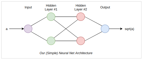
We randomly sampled 1000 positive numbers and took their square roots, split those pairs into ten batches, and trained the model for 1000 epochs. As expected, the model performed very well. As the model ran through its training epochs, the difference between the predicted value and the actual value went near to zero very quickly:

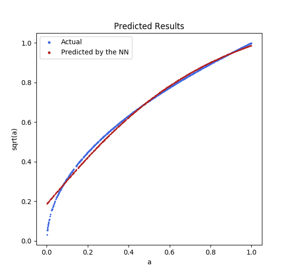
The results were mostly accurate, with some drift around the ends. So far, so good.
Kicking it up a Notch
Having cleared the first hurdle, we can now move on to solving the quadratic formula. To make our life a little simpler, we can ignore a, since it can always be scaled to one. To get training data, we could generate pairs of b and c and discard them if b² ≥ 4c. But there’s a more elegant way to do it: if the roots of our function are r₁ and r₂, then:
p(x) = (x – r₁)(x – r₂)
p(x) = x² – (r₁ + r₂)⋅x + r₁⋅r₂
so:
b = -(r₁ + r₂) and c = r₁⋅ r₂
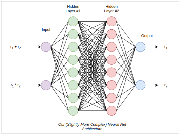
This means that we can sample r₁ and r₂ and make training pairs comprised of (r₁ + r₂, r₁⋅ r₂) as the input and (r₁, r₂) as the target output.
We’ll make our neural net architecture more complex, both because the space is more complicated and our input and output are different:
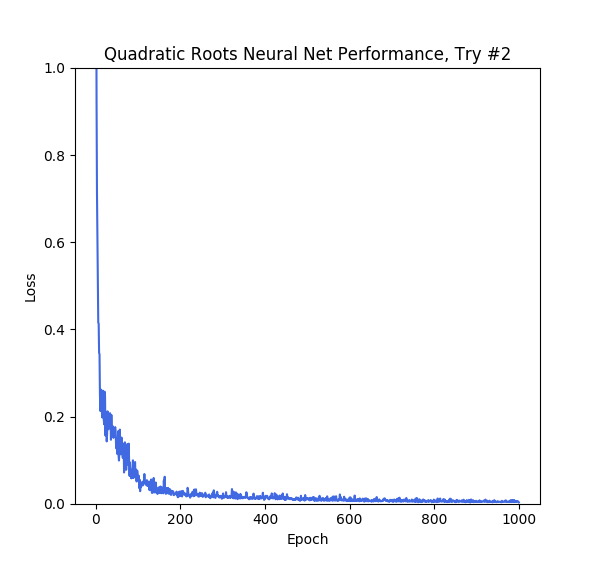
So, now all that remains is train the net and see how it does. The quadratic formula is a more complicated function than square roots, but ultimately it’s still pretty trivial, so we expected similar results. Here’s what we got:
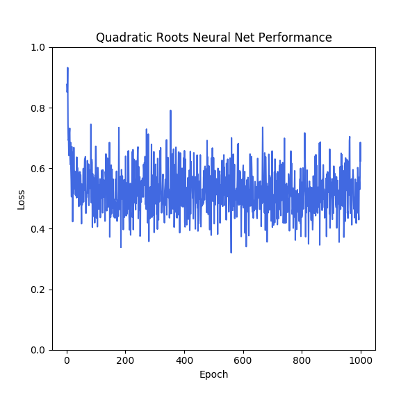
Results are pretty lackluster: the model error hits 0.5 around and then bounces around that figure for a while, sometimes lower, sometimes higher, but never making real progress.
So what went wrong? Well, when we trained the model, we acted as if the order of r₁ and r₂ didn’t matter, since we passed them through in an arbitrary manner. After all, this makes mathematical sense. Both (r₁, r₂) and ( r₂, r₁) are valid answers for (r₁ + r₂, r₁⋅ r₂).
To the model, however, the order does matter. That’s something baked into how models work; the first output and second output are distinct things, not interchangeable. This is what hurts model performance.
There’s an easy fix to this: just add order to the data. We can do this by adding in min and max functions to the targets, like this:
(r₁ + r₂, r₁⋅ r₂) → (min(r₁, r₂), max(r₁, r₂))
This imposes order on the output. The smaller root comes first, than the larger root. This in turn allows the model to train on the data:
The Bigger Picture
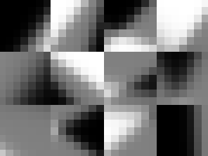
The motivating example for this experiment came from an issue that one of our data scientists ran into while working on a research effort. He was looking into convolutional neural nets and investigating the mathematical structure of images, towards the goal of improving and compacting embedding spaces. (An embedding space is the raw output of a neural net before classification occurs; the relative position of points in this space can inform us about the data.) As a start, he looked at images that were comprised of a line drawn an an angle, and intensity to shade the area under that line.

Each image was constructed from three variables, a and b, which defined the slope and intercept of the line, and c, which defined the intensity under the line. Each variable was randomly sampled between -1 and 1 (if c was negative, the area above the line would be shaded). A convolutional neural net was then trained on the images and was successfully used to calculate the values of a, b and c. Such reductions are potentially useful for reducing images down for quicker identification and processing.
However, when he tried the same technique on images with two lines laid over each other, model performance cratered.
The problem was the same one we just demonstrated with the quadratic formula: both lines mix together in the final image, but the model treats the order of those lines important when it actually isn’t. So, in order to learn this space, we needed to transform the parameters input to the model, so that they are order invariant. Once solved, we could train on CNNs to learn these compact embeddings for simple images; these embeddings could in turn be used for large scale image classification.
While these images are very simple, a similar transformation could be done on higher resolution images to create embeddings that represent the geometry of an image in just a few values, allowing for quicker classification and segmentation. With this technique, we can efficiently train convolution neural nets to learn compact embeddings for images in a completely unsupervised manner, and, as a bonus, we can even learn the quadratic formula.