Don’t Miss Your Turn: Calculating Aircraft Turn Locations from Trajectory Data
With the increasing availability of network connected GPS devices, aircraft trajectory data is now quite common. Mining trajectory data for patterns presents a number of unique challenges:
- Density: Trajectories are often represented as a collection of observations ordered by time. They are dense because, where traditional data sets would have a single observation, trajectories have several.
- Non-stationarity: Trajectories often change over time without clearly delineated shifts. This makes it difficult to characterize and compare data via traditional statistics.
- Time Warping: Trajectories often describe identical behavior occurring at different speeds. This can cause bias because slower trajectories often have more observations.
Below, we share a recent use case where we analyzed flight trajectories from commercial airline flights in order to automatically find significant heading changes. We used a combination of signal processing and machine learning to deal with the above three challenges. There is nothing that we found that a dedicated analyst couldn’t find. The real novelty of this work is the scale and speed at which we can find these patterns.
Problem
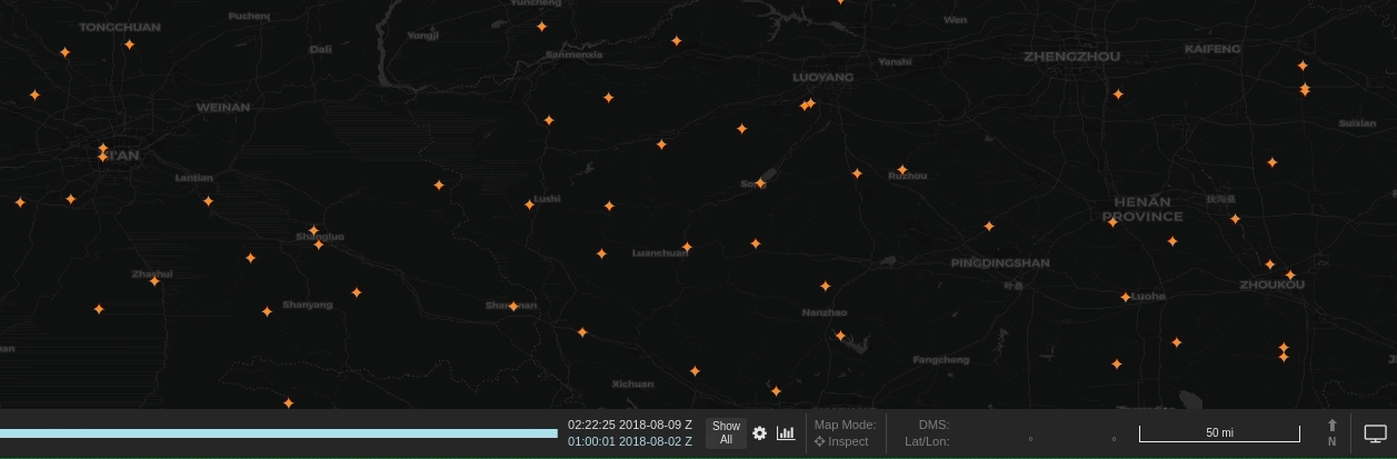
We wanted to identify locations where aircraft commonly turn, given point-in-time observations from worldwide aircraft flight paths.
Approach
With any machine learning project there are, in general, two ways to proceed: supervised or unsupervised. Given the characteristics of our trajectory data, supervised learning seemed like a poor approach. The volume and density of the data would make it difficult to create representative labeled features, and the non-stationary and time warping nature of the data would make it difficult to learn representative input features.
At the same time, a fully unsupervised approach also didn’t seem like a good idea. A fully unsupervised approach would likely do well to cluster and fit the data, but it would give little direction on how to evaluate the results or iteratively improve the underlying model.
In the end we used a semi-supervised approach. To fit the data—and all the oddities it might contain—we used an unsupervised method: mean shift clustering. Then, to evaluate the model, we created a small sample of obvious heading change locations. From these we could determine an approximate guess of precision and recall for the learned mean shift clusters.
Mean Shift Clustering
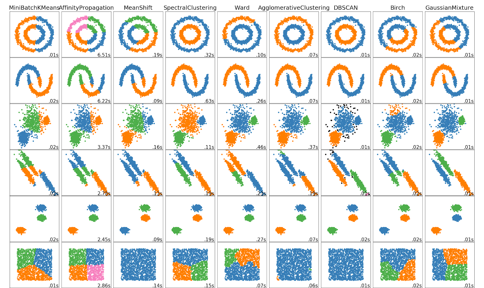
To get a feel for mean shift clustering, and why we chose it over other unsupervised methods, we can look at the scikit-learn example image to see the results of various clustering algorithms on test data (algorithm names are listed across the top of the image).
First, we wanted a method where the number of clusters wasn’t a parameter of the model. Given one week of world-wide commercial aircraft trajectories, predicting the correct number of turning clusters seemed undoable. This very quickly narrowed the field to DBSCAN and mean shift.
To understand the implications of this choice we can look at the last row in the cluster samples. The methods that use cluster count as a parameter find that number of clusters in the square data—despite the square, for our purposes, being a single cluster (e.g., Mini-batch k-means in the first column finds three clusters in the square). The all-blue squares at the bottom of those columns show that only mean shift and DBSCAN identify the square as a single cluster.
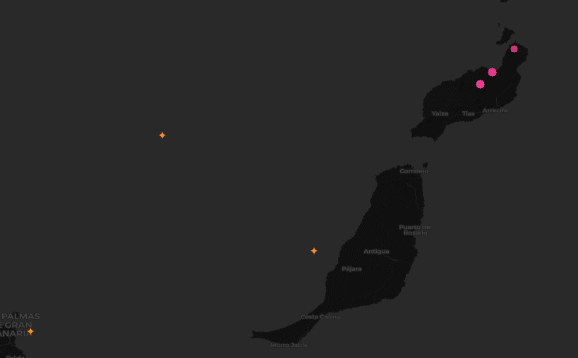
Next, we wanted a method which learned a centroid. The idea here was that, for any given turning location, aircraft would be observed at different points of their turn rather than exactly on the location. By finding the centroid of these observations, no single observation had to be the perfect representation of the turn. Instead we could use many observations from separate trajectories to get a much better estimate.
With these two requirements, mean shift was the only choice. Unfortunately, according to scikit-learn, mean shift doesn’t scale as well as other clustering methods. To address this we made a few modifications to the algorithm (detailed below) to get acceptable performance.
Data Pre-processing
To prep such a large amount of data we used Spark to parallelize computation. We were interested in two things:
- Removing potential sensor errors from the data
- Selecting only the data that was relevant to the task
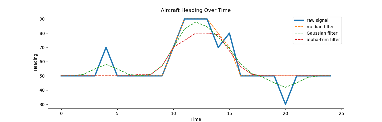
To remove errors from the data we looked to signal processing. The field of signal processing has a large collection of error correction tools called filters. These were originally designed for real-time electronic signals such as phone calls, but have been adapted to many other contexts since then. Most of the basic filters are easily implemented in a Spark query. The three we tested were a Gaussian filter, a median filter and an alpha-trim filter. Below we provide a figure that shows how these three filters would change the input of a theoretical data feed.
After applying the filter, we then wanted to narrow down the data to only observations that indicate that a turn is occuring. In fact, by clustering over all individual observations that are involved in a turn, rather than first trying to summarize a turning sequence in a trajectory as a single “turn”, we can work around the time warp challenge. That is, we are now working with single observations, rather than tracks.
To narrow the data, we used Spark DataFrame window functions (also known as analytic functions in SQL). These functions allow data to be sorted and partitioned in a single pass so that an observation can be compared to its immediate predecessor. This let us quickly find all the locations in a trajectory where an aircraft’s heading changed.
Mean Shift Speed Modifications
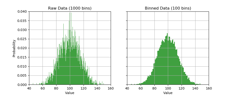
Because mean shift clustering typically doesn’t scale well, we sought to bound the size of N2 (where N is the number of data points) in order to control our run time. To do this we reduced the full observation set down to a smaller set of evenly spaced bins. We then used scikit-learn’s Kernel Density Estimators to assign a weight to each bin. The following shows how KDE binning can reduce 1000 observations to 100.
Mean Shift Accuracy Modifications
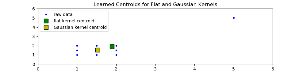
The mean shift implementation in scikit-learn uses a flat average of neighbors (sometimes referred to as a flat kernel). This approach works well if training data is dense at all clusters. Unfortunately, given that our data was for the whole globe and included high and low traffic turning points, this assumption didn’t seem right.
To improve our model’s accuracy, we replaced scikit-learn’s flat kernel with a Gaussian kernel that is less sensitive to outliers. The graph below shows raw input data containing an outlier and how mean shift’s centroid changes for a flat kernel and a Gaussian kernel.
Results
The end result was an algorithm that used a median filter up front to clean the data, followed by KDE binning to reduce the amount of data and finally a Gaussian weighted mean to give more robust statistics. For the data set we describe above the entire end-to-end process takes 40 minutes to complete, and we feel the results speak for themselves. Our final model found turning locations 42 times more frequently than random guessing alone while missing only half as much.