Interactive Insights into Hurricane Harvey’s Impact on Energy Production with GeoMesa & Zeppelin Notebooks
In the current Big Data environment, it’s crucial to have a quick iteration cycle for exploring data, performing analytics, and visualizing the result. For example, the impact of Hurricane Harvey on oil and gas shipping in the Gulf of Mexico last fall has many dimensions to explore, and plenty of data is available to use in this exploration is available, but the cost of running a cluster that can load and query large volumes of such data can be both financially expensive and time consuming.
Fortunately, modern cloud hardware lets us store data in a way that is both quick to access and cost effective. GeoMesa’s File System Datastore provides the ability to store spatio-temporally indexed data on Amazon S3 storage for pennies per GB/month. When we want to perform analysis, we can start up an ephemeral cluster to query the data and shut it down when complete. Using GeoMesa’s Spark integration also lets us harness Zeppelin notebooks and SparkSQL to provide quick analytics development and visualization. (For more on GeoMesa’s support for Zeppelin and Spark SQL, see last year’s blog entry New in GeoMesa: Spark SQL, Zeppelin Notebooks support, and more.)
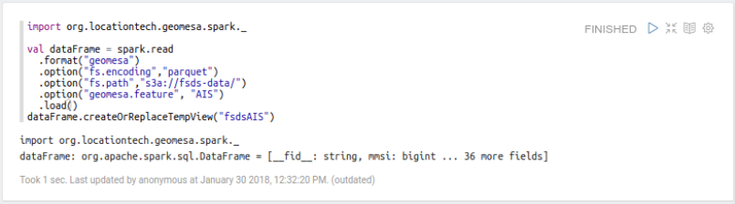
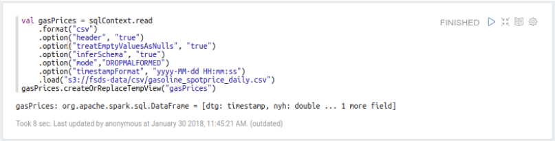
Let’s take a look at a recent data exploration workflow we performed to see how developments in tooling have changed the big data analytics landscape. Using the Geomesa FileSystem Datastore (FSDS), we have loaded over 10TB of Automatic Identification System (AIS) data from the data service company exactEarth into S3. The data is indexed by date with two bits of precision for the spatial index to break the world into quadrants. This produces files on the order of 100MB (after compression) when using Apache’s Parquet encoding. Taking advantage of Amazon’s EMR managed cluster platform, we can spin up a cluster with Spark and Zeppelin pre-installed and place the FSDS runtime on the Zeppelin Spark interpreter’s classpath. Connecting to the FSDS is then straightforward. Using the Scala interpreter in a Zeppelin notebook, we can obtain a GeoMesa-backed DataFrame which we’ll use to access our data. We also create a Temp View of the data that allows us to access it using Zeppelin’s SQL interpreter.
We’re now ready to work with the data. As a motivating example, hurricane Harvey shut down a lot of oil refineries in Houston, TX. Using SparkSQL, what information we could gather from the activity of tankers in the area around Houston during the hurricane?
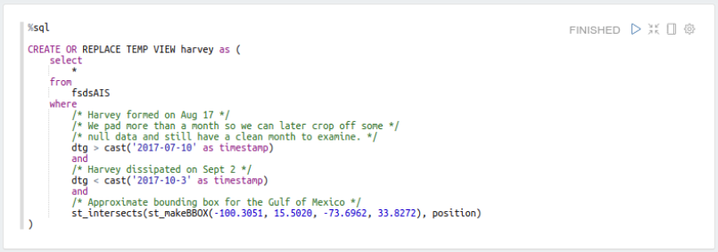
Selecting the dates around Harvey, padded by about a month, and constructing a bounding box around the Gulf of Mexico, we’ll create a temp view of the data to simplify later queries:
We can also cache the data in memory, if our cluster is large enough, to speed up queries:

Now let’s look at the number of tankers in the Gulf, by day. The SparkSQL query below retrieves the relevant data and then uses Zeppelin’s built-in graphing tools to graph the data over time:
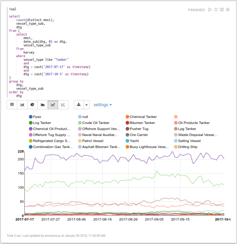
Unsurprisingly, this isn’t very interesting; despite the hurricane, the average number of ships shouldn’t change much since most ships will just avoid the affected area. However, this query only took about five seconds to run, showing the performance that this configuration is capable of.
Next, let’s adjust our query to give us more insight into what’s happening around Houston. This query buffers a point in Trinity Bay, just outside of Houston, by 50 km to capture the activity in and around Houston ports:
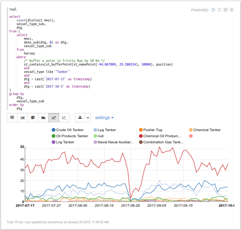
Harvey made landfall just south of Houston on Aug 26, 2017, and we can clearly see most of the tankers in the area leaving the day or two before. As interesting as this is, it’s not very useful by itself, so let’s pull in another dataset. After retrieving daily gasoline price data from EIA.gov and storing it in a comma-separated value file on S3, we load this data as well:
This data contains daily prices, in USD, from two gasoline price indexes: New York Harbor (nyh) and U.S. Gulf Coast (usgc). Let’s take a look at the data over the same time period:
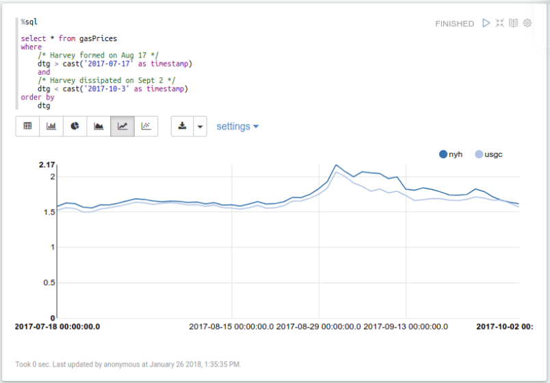
There is a very clear price spike in both indexes just after Harvey. Next, we’ll perform a Min/Max Normalization of both datasets and put them on the same graph so that we can see them together. To do this, we’ll break the query up into chunks that are easier to read.
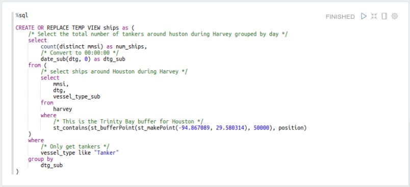
First gather the number of tankers in our area of interest, grouped by day:
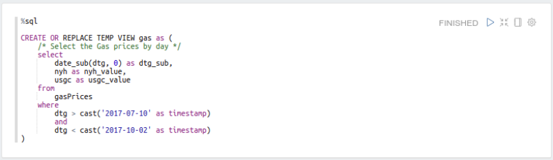
Then get the daily gas prices for our time range:
Next, join the tables together by date, back-filling any of the missing gas data with the previous day’s, and compute the Min/Max normalization:
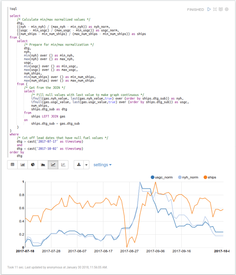
We can now clearly see the temporally delayed relationship between the number of tankers in the area and fuel prices. Performing additional analysis on this data and relationship is certainly possible, but extracting actionable analytics would be difficult without additional data. While there is definitely a correlation between the drop in crude oil deliveries being made and the increase of gasoline prices, this relationship is only part of the cause. Nevertheless, being able to quickly view this relationship and prototype analytics on top of it is valuable.
Querying the 10TB of data and performing this analysis took very little time, required very little DevOps, and, because we used Amazon’s Spot Pricing, was very inexpensive. From start to finish, standing up the Spark cluster, configuring Zeppelin, and running these analytics can easily be done in 15 minutes. At current spot prices and using Amazon’s Instance Hour billing structure, the total cost of this 8 node cluster (1 Master and 7 Workers) was $0.48 (64 normalized instance hours). This does not include the storage cost, but even this is much less than more traditional methods such as HDFS that require high replication factors and additional servers.
This exploration of AIS data gives you an idea of the how the interactive use of Zeppelin notebooks and SQL, combined with powerful tools such as Spark analytics and GeoMesa’s spatio-temporal capabilities, can let you quickly explore relationships between locations and time periods to provide more insight into unfolding events. The simple introduction of historical gasoline pricing data into the exploration showed how easy it is to mix and match different data sources to gain deeper insights.
What kinds of data would you like to mix and match with your spatio-temporal data to gain new insights? If you’re interested in maritime domain analytics and insights specific to your use case that can be derived from our historical archive of AIS data from exactEarth, let us know at info@optix.earth.