Rooting Out Routes

Problem

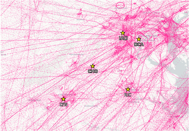
Rather than simply flying straight from point A to point B, commercial airline flights fly along preset routes. Pilots often liken these routes to “highways in the sky.” However, unlike highways on the ground, exact maps of these routes are hard to come by. While some countries make their charts available for free, not all do. Even maps that are available aren’t necessarily in a GIS-friendly, machine-readable format.

Also, unlike highways, these routes are flexible. They are constantly shifting as air traffic controllers adjust to day-to-day differences in traffic and weather. The set routes also change as air traffic grows and new airports open up. This makes finding a complete map of these routes impossible to gain access to.

While data on the routes is difficult to obtain, data on the planes flying them is not. We set out to work backwards, taking the raw data of planes on the route and deducing what routes those planes are following.

Data

The data we worked with is called Automatic Dependent Surveillance – Broadcast, or ADS-B. This data consists of point-in-time locations reported by planes, along with accompanying metadata such as groundspeed and altitude. Any commercially registered aircraft, from two-seater Cessnas to helicopters to transatlantic airliners, is included in this data. This data is picked up by commercially available receivers around the world. Coverage is widespread, but gaps exist, particularly over oceans and in developing countries. Our project used a week of ADS-B data totalling 184 million unique points.

Rollup

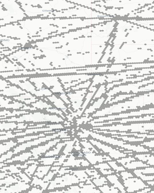
We had an Apache Spark cluster with GeoMesa set up to run calculations, but in order to aggregate these points into a more manageable size, we used the h4 library developed by Uber. h4 divides the earth into hexagonal cells of equal area, each of which has a unique hash value. h4 can associate points to those hashes, creating a key to use when aggregating the trajectory data we’re working on.

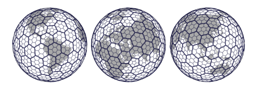
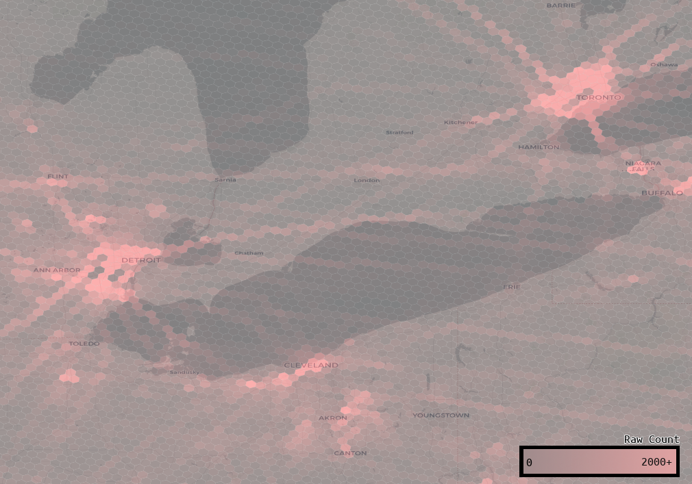
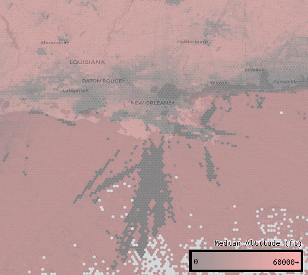
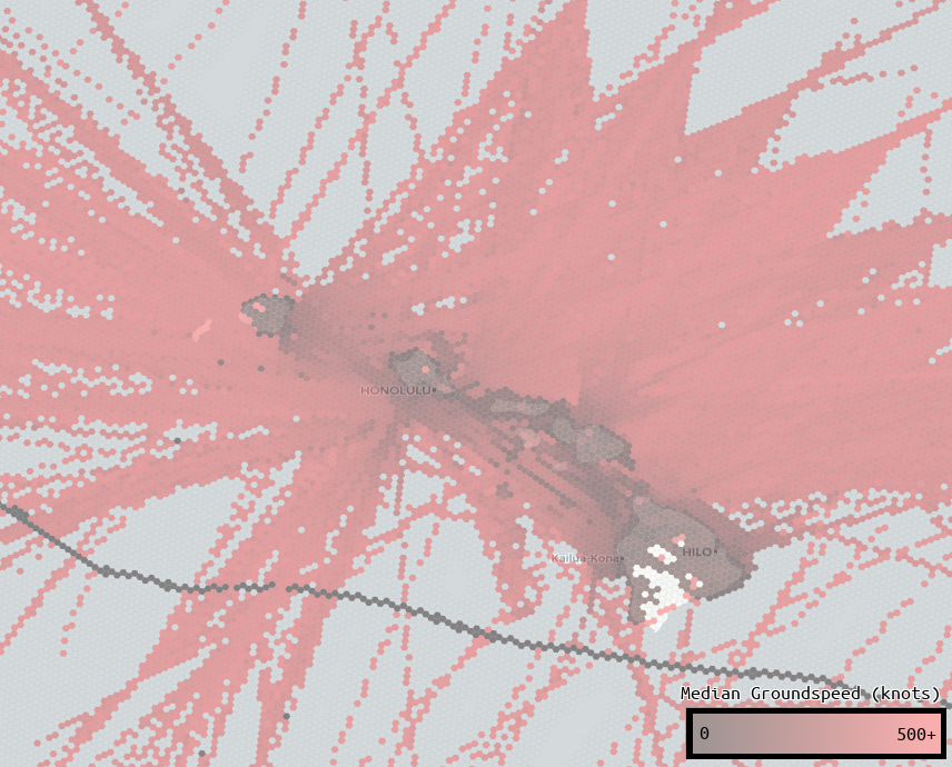
Using h4, we can associate each airplane point observation to a cell. Once associated by cell, we can aggregate that data in many different ways. This lets us categorize and examine different airspaces and find all sorts of interesting trends:

Raw count of observations over Lake Erie; denser pink coloring shows airports and routes

Median aircraft altitude per cell over New Orleans. Helicopters servicing oil rigs carve low altitude paths across the otherwise lofty altitudes of gulf aircraft

Median groundspeed per cell over Hawaii. Incoming transoceanic flights contrast with inter-island flights and sightseeing helicopters

Convolution

This problem was very frustrating because at first glance, the routes are right there! Anyone with eyes can easily pick them out. But choosing the perfect threshold for what defines a “route” is impossible, because routes vary wildly in traffic level. If you set a threshold based on busy areas, less travelled routes will not have enough traffic to be recognized. If you set your threshold too low, you’ll wash out obvious routes in areas with more activity.

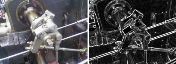
The same area, with two different thresholds.These show radically different routes, neither of them particularly useful.

In order to fix this, we borrowed a technique from image processing. We were inspired by edge detection algorithms such as the Sobel operator. The Sobel operator sets pixel values based on the surrounding pixels. The less like its neighbors a pixel is, the higher its value will be post-Sobel.

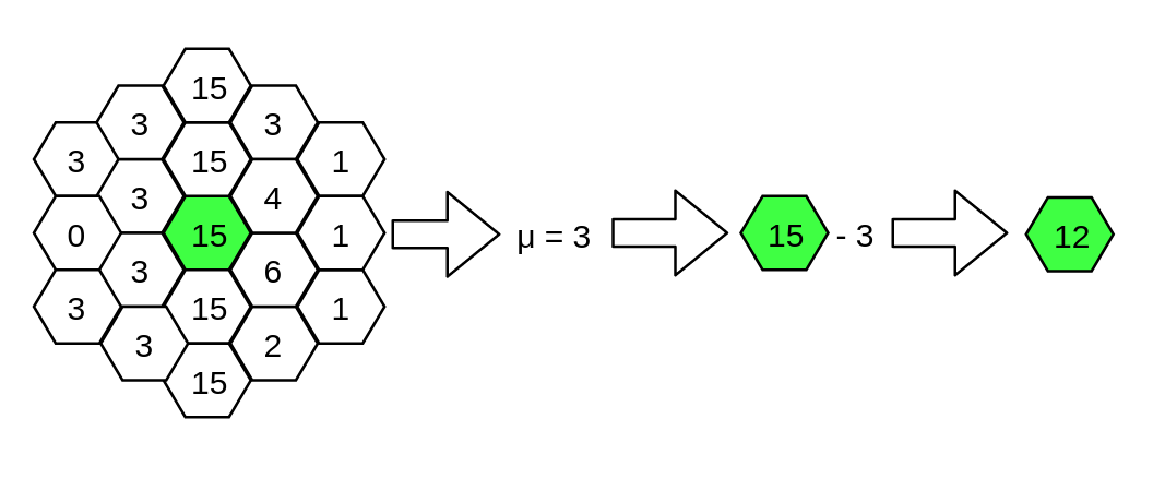
The Sobel operator in action (Provided by Simpsons Creator via CC BY-SA 3.0)

To achieve something similar with the h4 cells, we applied a median filter to the hexagons, which took the median value of the surrounding hexagons. We then subtracted that value from the aircraft count in the cell.

Take the example below, where the cell the filter is running on is highlighted in green. In this case, the filter is calculated with a radius of two. The median for all cells within two jumps is calculated, and it ends up being three. So, three is subtracted from the cell, giving us a new value of twelve.

This helped us find local peaks and valleys in the value set, with the peaks as routes, and the valleys and plains as non-routes. Cells with significantly higher values than the cells around them stick out from the rest. We could then pick a good threshold and separate routes and non-routes.

Results

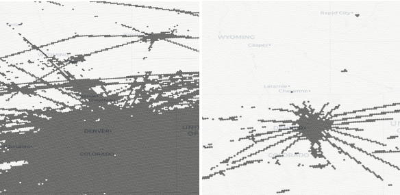
With this method, we were able to recreate routes worldwide:

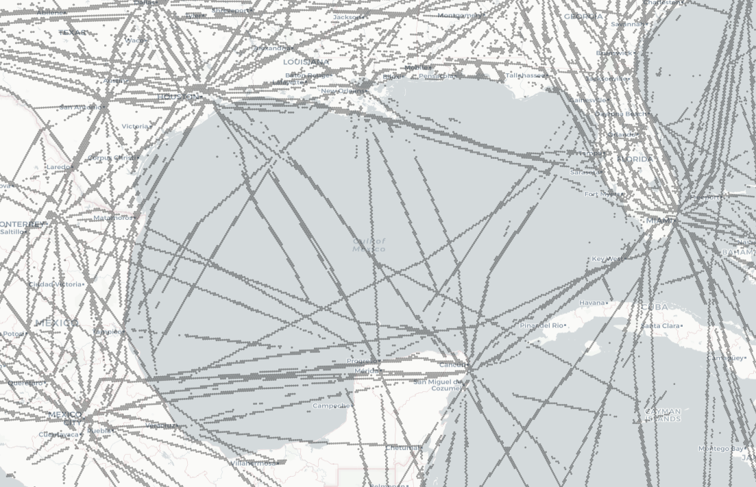
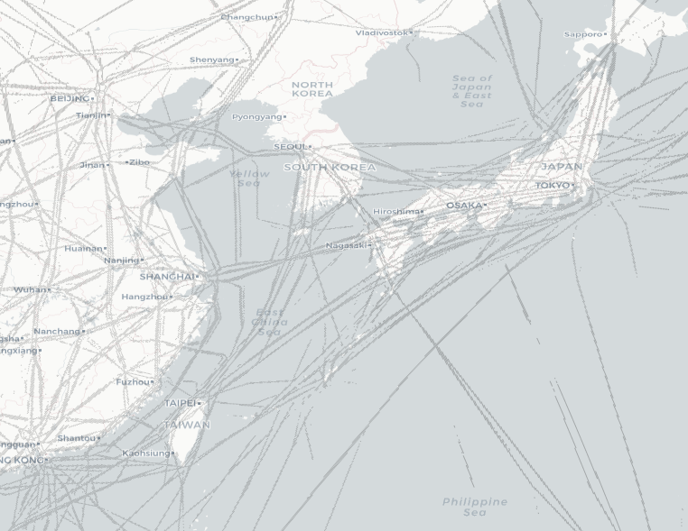
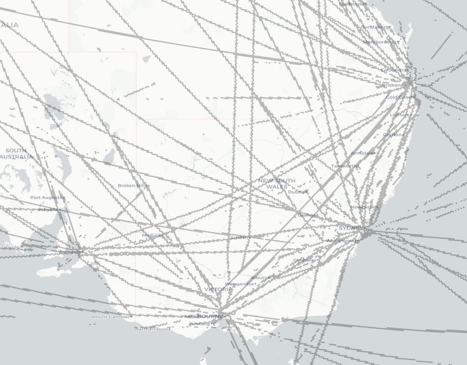
Overall, the results are pretty good. We captured routes on a global scale using data from the planes actually flying them. There are a few annoying gaps—in particular, when two routes overlap, the less-travelled route would often get overshadowed by the more frequently travelled one. But for the most part, this method provides a map of routes that planes actually fly, and it can be easily recreated as those routes change.

Go Back